My first go at writing an application in Rust has been slightly frustrating. Coming in from using mostly dynamic languages every day I quickly found myself butting heads with Rust’s borrow checker. However, I’ve found that this is a fair price to pay for a statically typed language with a focus on memory safety and performance.
While these Rust features do increase the barrier of entry for newcomers such as myself, they also help to keep your code in check and are certainly major contributing factors to the language’s success.
Another interesting point is that Rust doesn’t have a GC (garbage collector). As soon as something in your code is not required anymore (a function call returns) the memory associated with that scope is cleaned up. Rust inserts Drop::drop calls at compile time to do this. I imagine this is similar in concept to the way that IL or code weaving is done in the .NET world. This fact means that Rust doesn’t suffer from performance hits that languages with a GC tend to sometimes encounter. Discord wrote an interesting article on how they improved performance by switching from Go to Rust that touches on this particular point.
Goals
To take a look at the Rust language and ecosystem at a really high-level, I decided to write a simple tool. My goals were to:
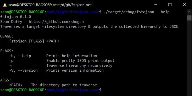
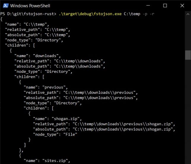
Write a CLI tool, small in scope. The tool will traverse a target directory in the file system recursively and print the structure to stdout as JSON.
Get a feeling for the language’s syntax.
See how package management and dependencies work.
Look at what the options are for cross-compiling to other platforms.
The tool – fstojson
Here is the small tool I wrote to achieve the above list of goals: fstojson-rust.
I’ve compiled my first app on macOS, Linux and Windows all from the same source, with no issues whatsoever.
Rust Packages
On my first look at Rust, packages were simple to understand and use. Rust uses “crates” and they work very similarly to JavaScript packages.
To add a crate to your project you simply add the dependency to your Cargo.toml file (akin to a package.json file in Node.js).
For example:
[dependencies]
serde_json = "1.0.68"
Once crates are installed with the cargo command, you’ll even get a lock file (Cargo.lock), just like with npm or yarn in a Node.js project.
Rust cross compiling
The first time you install Rust with rustup, the standard library for your current platform is installed. If you want to corss compile to other platforms you need to add those target platforms seperately.
Use the rustup target add command to add other platform targets. Use rustup target list to show all possible targets.
To cross-compile you’ll often also need to install a linker. For example if you were trying to compile for x86_64-unknown-linux-gnu on Windows you would need the cc linker.
Thoughts and impressions
To get a really simple “hello-world” application up and running in Rust was trivial. The cargo command makes things really easy for you to scaffold out a project.
However, I honestly struggled with anything more complex for a couple of hours after that. Mostly fighting the “borrow checker”. This is my fault because I didn’t really spend much time getting acquainted with the language initially via the documentation. I dove right in with trying to write a small app.
The last time I wrote something in a System programming language was at least 7 or 8 years ago – I wrote a tool in C++ to quiesce the file system in preparation for snapshots to be taken. Aside from that, the last time I really had to concern myself with memory management was with Objective-C (iOS), before ARC was introduced (See my first serious attempt at creating an iOS game, Cosmosis).
In my opinion, some of Rust’s great benefits also mean it has a high barrier of entry. It has a really strong emphasis on memory safety. I came at my first application trying to do all the things I can easily do in Typescript / Javascript or C#.
I very quickly realised how different things are in the Rust world, and how this opinionated approach helps to keep your code bug-free and your apps safe on memory.
Closing thoughts
After years of dynamic language use, my first introduction to Rust has been a little bit shaky. It’s a high barrier of entry, but with that said, I did find it satisfying that if there were no compiler warnings my code was pretty much guaranteed to run without issue.
The Rust ecosystem is active and thriving from what I can tell. You can use crates.io to search online for packages. You can use rustup to install toolchains and targets.
There are tons of stackoverflow questions and answers and the documentation page for Rust is full of good information.
Going forward I’ll try to dig into the Rust language a bit more. I’m on a little bit of a journey to try different programming languages (I’ve had a fair bit of experience in C# and Typescript / JavaScript, so I’m branching out from those now).
I discovered this post recently – A half-hour to learn Rust. In hindsight it would have been great to have found that before diving in.
Recently I’ve been playing around with Ultimate Packer for Executables (UPX) to reduce a distributable CLI application’s size.
The application is built and stored as an asset for multiple target platforms as a GitHub Release.
I started using UPX as a build step to pack the executable release binaries and it made a big difference in final output size. Important, as the GitHub Release assets cost money to store.
UPX has some great advantages. It supports many different executable formats, multiple types of compression (and a strong compression ratio), it’s performant when compressing and decompressing, and it supports runtime decompression. You can even plugin your own compression algorithm if you like. (Probably a reason that malware authors tend to leverage UPX for packing too).
In my case I had a Node.js application that was being bundled into an executable binary file using nexe. It is possible to compress / pack the Node.js executable before nexe combines it with your Node.js code using UPX. I saw a 30% improvement in size after using UPX.
UPX Packing Example
Let’s demonstrate UPX in action with a simple example.
Create a simple C application called hello.c that will print the string “Hello there.”:
#include "stdio.h"

int main() {
  printf("Hello there.\n");
  return 0;
}
Compile the application using static linking with gcc:
gcc -static -o hello hello.c
Note the static linked binary size of your new hello executable (around 876 KB):
sean@DESKTOP-BAO9C6F:~/hello$ gcc -static -o hello hello.c
sean@DESKTOP-BAO9C6F:~/hello$ ls -la
total 908
drwxr-xr-x  2 sean sean   4096 Oct 24 21:27 .
drwxr-xr-x 26 sean sean   4096 Oct 24 21:27 ..
-rwxr-xr-x  1 sean sean 896336 Oct 24 21:27 hello
-rw-r--r--  1 sean sean  23487 Oct 21 21:33 hello.c
sean@DESKTOP-BAO9C6F:~/hello$
This may be a paltry example, but we’ll take a look at the compression ratio achieved. This can of course, generally be extrapolated for larger file sizes.
Analysing our Executable Before Packing
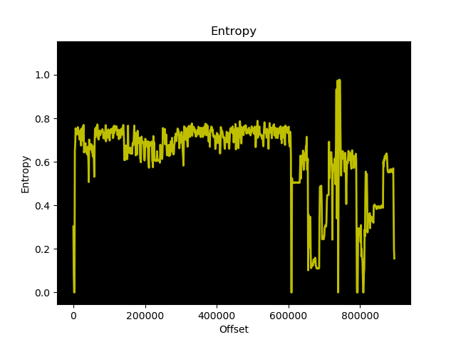
Before we pack this 876 KB executable, let’s analyse it’s entropy using binwalk. The entropy will be higher in parts where the bytes of the file are more random.
Generate an entropy graph of hello with binwalk:
binwalk --entropy --save hello
The lower points of entropy should compress fairly well when upx packs the binary file.
UPX Packing
Finally, let’s pack the hello executable with UPX. We’ll choose standard lzma compression – it should be a ‘friendlier’ compression option for anti-virus packages to more widely support.
upx --best --lzma -o hello-upx hello
Look at that, a 31.49% compression ratio! Not bad considering the code itself is really small and most of the original hello executable size is a result of static linking.
sean@DESKTOP-BAO9C6F:~/hello$ upx --best --lzma -o hello-upx hello
                       Ultimate Packer for eXecutables
                          Copyright (C) 1996 - 2020
UPX 3.96        Markus Oberhumer, Laszlo Molnar & John Reiser   Jan 23rd 2020

        File size         Ratio      Format      Name
   --------------------   ------   -----------   -----------
    871760 ->    274516   31.49%   linux/amd64   hello-upx

Packed 1 file.
sean@DESKTOP-BAO9C6F:~/hello$
Running the packed binary still works perfectly fine. UPX cleverly re-arranges the binary file to place the compressed contents in a specific location, adds a new entrypoint and a bit of logic to decompress the data when the file is executed.
UPX is a great option to pack / compress your files for distribution. It’s performant and supports many different executable formats, including Windows and 64-bit executables.
A great use case, as demonstrated in this post is to reduce executable size for binary distributions, especially when (for example) cloud storage costs, or download sizes are a concern.
A while ago I read a fantastic article by Alex Bainter about how he used markov chains to generate new versions of Aphex Twin’s track ‘aisatsana’. After reading it I also wanted to try my hand at generating music using markov chains, but mix it up by tring out alda.
‘aisatsana’ is very different to the rest of Aphex Twin’s 2012 released Syro album. It’s a calm, soothing piano piece that could easily place you into a meditative state after listening to it.
Alda is a text-based programming language for music composition. If you haven’t tried it before, you’ll get a feel for how it works in this post. If you want to learn about it through some much simpler examples, this quick start guide is a good place to start.
Generating music is made easier using the simple language that alda provides.
As an example, here are 4 x samples ‘phrases’ that are generated with markov chains (based off the aisatsana starting state), and played back with Alda. I’ve picked 4 x random phrases out of 32 that sounded similar to me, but were different in each case. A generated track will not necessarily consist of all similar sounding phrases, but might contain a number of these.
Markov Chains 101
On my journey, the first stop was to learn more about markov chains.
Markov chains are mathematical “stochastic” systems that change from one “state” (a situation or set of values) to another. In addition to this a Markov chain tells you the probabilitiy of transitioning from one state to another.
Using a honey bee worker as an example we might say: A honey bee has a bunch of different states:
At the hive
Leaving the hive
Collecting pollen
Make honey
Returning to hive
Cleaning hive
Defending hive
After observing honey bees for a while, you might model their behaviour using a markov chain like so:
When at the hive they have:
50% chance to make honey
40% chance to leave the hive
10% chance to clean the hive
When leaving the hive they have:
95% chance to collect pollen
5% chance to defend the hive
When collecting pollen they have:
85% chance of collecting pollen
10% chance of returning to hive
5% chance to defend the hive
etc…
The above illustrates what is needed to create a markov chain. A list of states (the “state space”), and the probabilities of transitioning between them.
To play around with Markov chains and simple string generation, I created a small codebase (nodejs / typescript). The app takes a list of ‘chat messages logs’ (really any line separated list of strings) as input. It then uses random selection to find any lines containing the ‘seed’ string.
With the seed string, it generates new and potentially unique ‘chat messages’ based on this input seed and the ‘state’ (which is the list of chat messages fed in).
Using a random function and initial filtering means that the generation probability is constrained to the size of the input and filtered list, but it still helped me understand some of the concepts.
Converting Aisatana MIDI to Alda Format
To start, the first thing I needed was a list of musical segments from the original track. These are what we refer to as ‘phrases’.
As Alex did in his implementation, I grabbed a MIDI version of Aisatsana. I then fed it into a MIDI to JSON converter, yielding a breakdown of the track into individual notes. Here is what the first two notes look like:
From there I wrote some javascript to take these notes in JSON format, parse the time values and order them into the 32 ‘phrases’ that aisatsana is made up of.
That is, there are 32 ‘phrases’, with each consisting of 32 ‘half-beats’ at 0.294117647058824 seconds per half beat. Totalling the 301 seconds.
const notes = [] // <-- MIDI to JSON notes here

// constants specific to the aisatsana track
const secPerHalfBeat = 0.294117647058824;
const phraseHalfBeats = 32;

// Array to store quantized phrases
let phrases = [];

notes.forEach(n => {
  const halfBeat = Math.round(n.time / secPerHalfBeat);
  const phraseIndex = Math.floor(halfBeat / phraseHalfBeats);
  const note = n.name.substring(0, 1).toLowerCase();
  const octave = n.name.substring(1, 2);
  const time = n.time;
  const duration = n.duration;

  // Store note in correct 'phrase'
  if (!phrases[phraseIndex]) {
  	phrases[phraseIndex] = [];
  }

  phrases[phraseIndex].push({ note: note, octave: octave, time: time, duration: duration });
});
It also gathers information such as the note symbol, octave, and duration for each note and stores it in a phrases array, which also happens to be ordered by phrase index.
Grouping by Chord
Next, the script runs through each phrase and groups the notes by time. If a note is played at the same timestamp, that means it is part of the same chord. To play correctly with alda, I need to know this, so a chords array is setup for each phrase.
phrases.forEach(phrase => {
  let chords = []
  const groupByTime = groupBy('time');
  phrase.chords = [];
  const chordGrouping = groupByTime(phrase);

  for (let [chordTimestamp, notes] of Object.entries(chordGrouping)) {
    phrase.chords.push(notes)
  }
});
Generating alda Compatible Strings
With chord grouping done, we can now convert the track into 32 phrases that alda will understand.
phrases.forEach(phrase => {
  let aldaStr = "piano: (tempo 51) (quant 90) ";
  phrase.chords.forEach(chord => {
    if (chord.length > 1) {
      // Alda plays notes together as a chord when separated by a '/'
      // character. Generate the alda string based on whether or not
      // it needs to have multiple notes in the chord, separating with
      // '/' if so.
      for (let [idx, note] of Object.entries(chord)) {
        if (idx == chord.length - 1) {
          aldaStr += `o${note.octave} ${note.note} ${note.duration}s `;
        } else {
          aldaStr += `o${note.octave} ${note.note} ${note.duration}s / `;
        }

      };
    } else {
      chord.forEach(note => {
        aldaStr += `o${note.octave} ${note.note} ${note.duration}s `;
      });
    }
  });
  // Output the phrase as an alda-compatible / playable string (you can
  // also copy this directly into alda's REPL to play it)
  console.log(aldaStr);
})
Here is the full script to convert the MIDI to alda phrase strings.
Generating Music with Markov Chains
There are different entry points that I could have used to create the markov chain initial state, but I went with feeding in the alda strings directly to see what patterns would emerge.
Here are the first 4 x phrases from aisatsana in alda-compatible format:
piano: (tempo 51) (quant 90) o3 e 0.5882355s o3 g 0.5882355s o3 c 0.5882354999999999s o4 c 7.6470615s
piano: (tempo 51) (quant 90) o3 e 0.5882354999999997s o3 g 0.5882354999999997s o3 c 0.5882354999999997s o4 c 0.5882354999999997s o3 b 2.3529420000000005s o4 e 4.705884000000001s
piano: (tempo 51) (quant 90) o3 e 0.5882354999999997s o3 g 0.5882354999999997s o3 c 0.5882354999999997s o4 c 0.5882354999999997s o3 b 7.058826s
piano: (tempo 51) (quant 90) o3 e 0.5882354999999997s o3 g 0.5882354999999997s o3 c 0.5882354999999997s o4 c 0.5882354999999997s o3 b 1.1764709999999994s o4 e 5.882354999999997s
If you like, you can drop those right into alda’s REPL to play them, or drop them into a text file and play them with:
alda play --file first-four-phrases.alda
The strings are quite ugly to look at, but it turns out that they can still be used to generate new and original phrases based off the aisatsana track phrases using markov chains.
Using the markov-chains npm package, I wrote a small nodejs app to generate new phrases. It takes the 32 x alda compatible phrase strings from the original MIDI track of ‘aisatsana’ as a list of states and walks the chain to create new phrases.
E.g.
const states = [
  // [ alda phrase strings here ],
  // [ alda phrase strings here ],
  // [ alda phrase strings here ]
  // etc...
]

const chain = new Chain(states);

// generate new phrase(s)
const newPhrases = chain.walk();
I threw together a small function that you can run directly to generate new phrases. Give it a try here. Hitting this URL in the browser will give you new phrases from the markov generation.
If you want a text version that you can drop right into the alda REPL or into a file for alda to play try this:
(Just add the instrument type, temp, and quant values you would like to the beginning of each line). E.g.
piano: (tempo 51) (quant 90) o4 (volume 30.71) e 0.5882354999999961s / o3 (volume 30.71) e 0.5882354999999961s o4 (volume 30.71) e 0.5882354999999961s / o3 (volume 31.50) g 0.5882354999999961s o4 (volume 30.71) d 0.5882354999999961s / o3 (volume 29.92) c 0.5882354999999961s o4 (volume 29.92) c 0.5882354999999961s / o3 (volume 31.50) e 0.5882354999999961s o3 (volume 29.92) b 7.0588260000000105s / o3 (volume 30.71) d 7.0588260000000105s
piano: (tempo 51) (quant 90) o4 (volume 30.71) e 0.29411774999999807s / o3 (volume 30.71) g 0.29411774999999807s o4 (volume 30.71) e 0.5882355000000032s / o3 (volume 30.71) e 0.5882355000000032s o4 (volume 30.71) d 0.5882355000000032s / o3 (volume 29.92) c 0.5882355000000032s o4 (volume 29.92) c 0.5882355000000032s / o3 (volume 31.50) e 0.5882355000000032s o3 (volume 29.92) b 7.058826000000003s / o3 (volume 30.71) d 7.058826000000003s
piano: (tempo 51) (quant 90) o4 (volume 30.71) e 0.29411774999999807s / o3 (volume 30.71) e 0.29411774999999807s o4 (volume 59.84) g 0.29411774999999807s o4 (volume 60.63) a 0.29411774999999807s / o4 (volume 30.71) e 0.5882354999999961s / o3 (volume 31.50) g 0.5882354999999961s o4 (volume 62.20) b 0.29411774999999807s o5 (volume 62.99) c 0.5882354999999961s / o4 (volume 30.71) d 0.5882354999999961s / o3 (volume 29.92) c 0.5882354999999961s o5 (volume 65.35) e 0.5882354999999961s / o4 (volume 29.92) c 0.5882354999999961s / o3 (volume 31.50) e 2.3529419999999845s o5 (volume 66.93) b 0.5882354999999961s / o3 (volume 29.92) b 1.7647064999999884s o5 (volume 60.63) g 8.823532499999999s o4 (volume 30.71) e 7.0588260000000105s / o2 (volume 30.71) c 7.0588260000000105s / o3 (volume 30.71) e 7.0588260000000105s
piano: (tempo 51) (quant 90) o4 (volume 30.71) e 0.29411774999999807s / o3 (volume 30.71) e 0.29411774999999807s o4 (volume 59.84) g 0.29411774999999807s o4 (volume 60.63) a 0.29411774999999807s / o4 (volume 30.71) e 0.5882354999999961s / o3 (volume 31.50) g 0.5882354999999961s o4 (volume 62.20) b 0.29411774999999807s o5 (volume 62.99) c 0.5882354999999961s / o4 (volume 30.71) d 0.5882354999999961s / o3 (volume 29.92) c 0.5882354999999961s o5 (volume 65.35) e 0.5882354999999961s / o4 (volume 29.92) c 0.5882354999999961s / o3 (volume 31.50) e 7.647061499999992s o5 (volume 66.93) b 0.5882354999999961s / o3 (volume 29.92) b 2.3529419999999988s o5 (volume 60.63) g 6.4705905s o4 (volume 15.75) e 4.7058839999999975s
I’ve uploaded the code here that does the markov chain generation using the initial alda phrase strings as input state.
Results and Alda Serverless
Generated Music
The results from generating music off the phrases from the original track are certainly fun and interesting to listen to. The new phrases play out in different ways to the original track, but still have the feeling of belonging to the same piece of music.
Going forward I’ll be definitely experiment further with markov chains and music generation using alda.
Experimenting with alda and Serverless
Something I got side-tracked on during this experiment was hosting the alda player in a serverless function. I got pretty far along using AWS Lambda Layers, but the road was bumpy. Alda requires some fairly chunky dependencies.
Even after managing to squeeze Java and the Alda binaries into lambda layers the audio playback engine was failing to start in a serverless function.
I managed to clear through a number of problems but eventually my patience wore down and I settled with writing my own serverless function to generate the strings to feed into alda directly.
My goal here was to generate unique phrases, output them to MIDI, and then convert them to Audio to be played almost instantenously. For now it’s easy enough to take the generated strings and drop them directly into the alda REPL or play them direct from file though.
It will be nice to see alda develop further and offer an online REPL – which would mean the engine itself would be light enough to perform the above too.
In the late ninetees, as a teenager I had the priveledge of owning a second hand Creative Labs 3dfx Voodoo 2 graphics card. It was an upgrade for my own hand-built PC – an AMD K6-2 333mhz system I had painstakingly saved up for and cobbled together.
Nostalgia running high, I recently set about building up a ‘retro’ gaming PC. With roughly the same specification as my original K6-2 machine from the late ninetees, it also features an original 3dfx Voodoo 2 accelerator card.
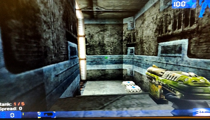
Unreal Tournament playing on my retro PC with the 3dfx Voodoo 2
The Brief Story of 3dfx Interactive and the Voodoo
A group of colleagues originally working together at SGI decided to break out and create 3dfx Interactive in San Jose, California (1994). This was after an initial failed attempt at selling rather pricey IrisVision boards for PCs.
Their original plan was to create specialist hardware solutions for arcade games, but they changed direction to instead design PC add-on boards. The reason for their pivot came about as a result of a few favourable factors. Namely:
The cost of RAM was low enough to make this a feasible endeavour.
RAM latency was much improved and allowed for ‘high’ clock speeds of up to 50MHz.
3D games were picking up in popularity. Spearheaded initially no doubt by id software with games such as Wolfenstein 3D, DOOM, the market was clearly headed to a point where 3D accelerated graphics would be in demand.
The first design, the SST1 (marketed as the Voodoo 1), targeted the $300-$400 price range for consumer PCs. A variety of OEMs picked up the design and released their own reference design boards, leading to the success of the original Voodoo line-up of 3D accelerator cards.
Enter the Voodoo 2
After the initial success of the Voodoo 1, the 3dfx Voodoo 2 (SST2) was soon born. It had vastly improved specifications over the original SST1 design such as:
100MHz clock rated EDO RAM (running at 90 MHz, 25 ns)
90MHz ASICs
2 x Texture Mapping Units (TMUs)
The fillrate of the Voodoo 2 was around 90 MPixels/s, and frame rates in benchmarks showed a massive uplift, nearly doubling in some cases.
My first (original) 3DFX Voodoo 2 PC Build
My first self-built (from scratch) PC was a bit of a frankenstein build. I had carefully budgeted and selected a motherboard that had onboard everything. Graphics, sound and networking. It would also run an AMD K6-2 CPU – a budget friendly option compared to Intel at that time.
The onboard graphics card shared 8MB of memory from system RAM (of which I only had 32MB total). As far as I recall it was capable of running Direct3D enabled games, albeit hobbling along with crippled frame rates.
Upgrading to a 3dfx Accelerator Card
After enduring this ‘fps hardship’ and learning more about the recently successful 3dfx graphics cards (a friend had a 4MB 3dfx Voodoo ‘1’ card), I found out about a second hand option. It was available through a friend of a friend, and would cost me 500.00 South African Rand (ZAR). This was a lot for a teen back then. I had saved up money, and bargained with my parents to combine my funds with a birthday gift contribution in order to purchase this card.
The Creative Labs 3D Blaster Voodoo 2. Mine came in almost identical packaging, but I had the 12MB version.
As I recall, I had to make massive concessions in order to fit the graphics card into my machine.
My motherboard only had 2 PCI slots. Both were horizontally in line with the CPU socket. The board design was probably never intended to house cards longer than the average PCI device at the time.
I had to remove the K6-2’s heatsink I was using and replace it with one from an older 486 machine that I had lying around. The profile of the 486 heatsink was much lower, allowing the 3dfx Voodoo 2 card to slot into a PCI slot, extending over the heatsink.
The problem now was that the 3dfx card’s lower PCB edge was now just about in direct contact with the heatsink. Another issue was that the heatsink was not made for mounting to a Socket 7 board. This forced me to lay my computer’s chassis down on it’s side in order for gravity to keep the heatsink in place!
I had a plan to keep pressure on the heatsink to maintain better contact with the CPU. Using a bit of non-conductive material between the 3dfx card’s PCB and the heatsink, I kept things in place. I also had to permanently angle a large fan blowing into the now open case.
This was the price I would pay to have my budget 3dfx voodoo 2 enabled system.
The Retro 3dfx Voodoo 2 PC Build
Recently after a bout of nostalgia and watching LGR videos, I started trawling eBay for old PC parts. The goal was to almost identically match my original PC build.
After a number of weeks of searching, I found the following parts. The motherboard was the most difficult to find (at a good price). Most Super Socket 7 boards I would find were dead and listed as spare parts.
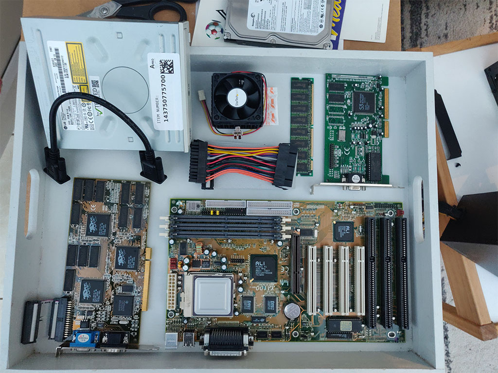
Most of the parts lined up and ready for the build.
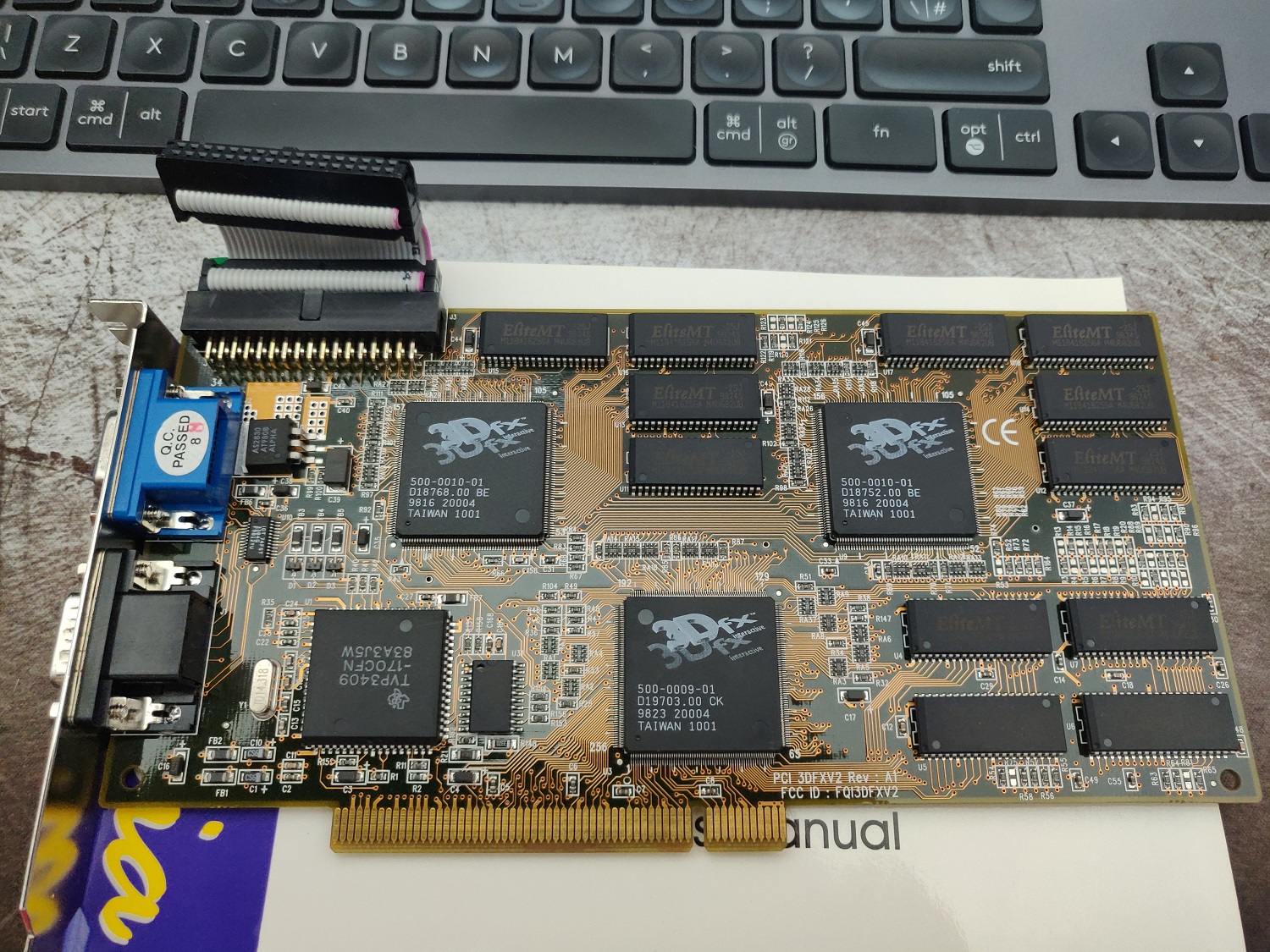
Iwill XA100 Aladdin V Super7 Motherboard, an AMD K6-2 300 CPU, and 64MB of PC100 SDRAM (168 pin)
S3 Trio 3D/2X graphics card (the Voodoo only handled 3D, and uses a loopback cable to plug into a ‘2D’ card)
3DFX JoyMedia Apollo 3D fast II 12Mb Video Card PCI Voodoo2 3DFX V2 Rev A1
A Retro styled, beige ATX PC Chassis, Computer MIDI Tower Case
Creative Sound Blaster Live 5.1 Digital SB0220 PCI Sound Card
An 80GB IDE HDD, IDE ribbon cable, and an older DVD-R drive.
I used a modern 80 plus certified ATX power supply. It has a power connector with an older 20 pin layout which was perfect to re-use.
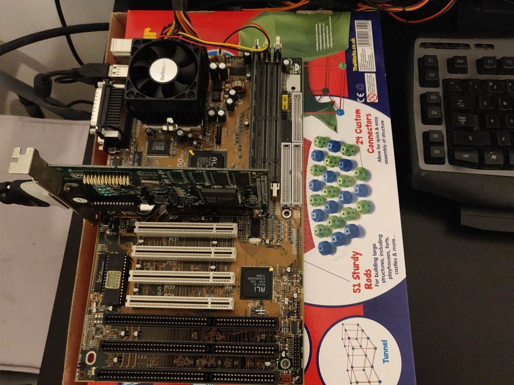
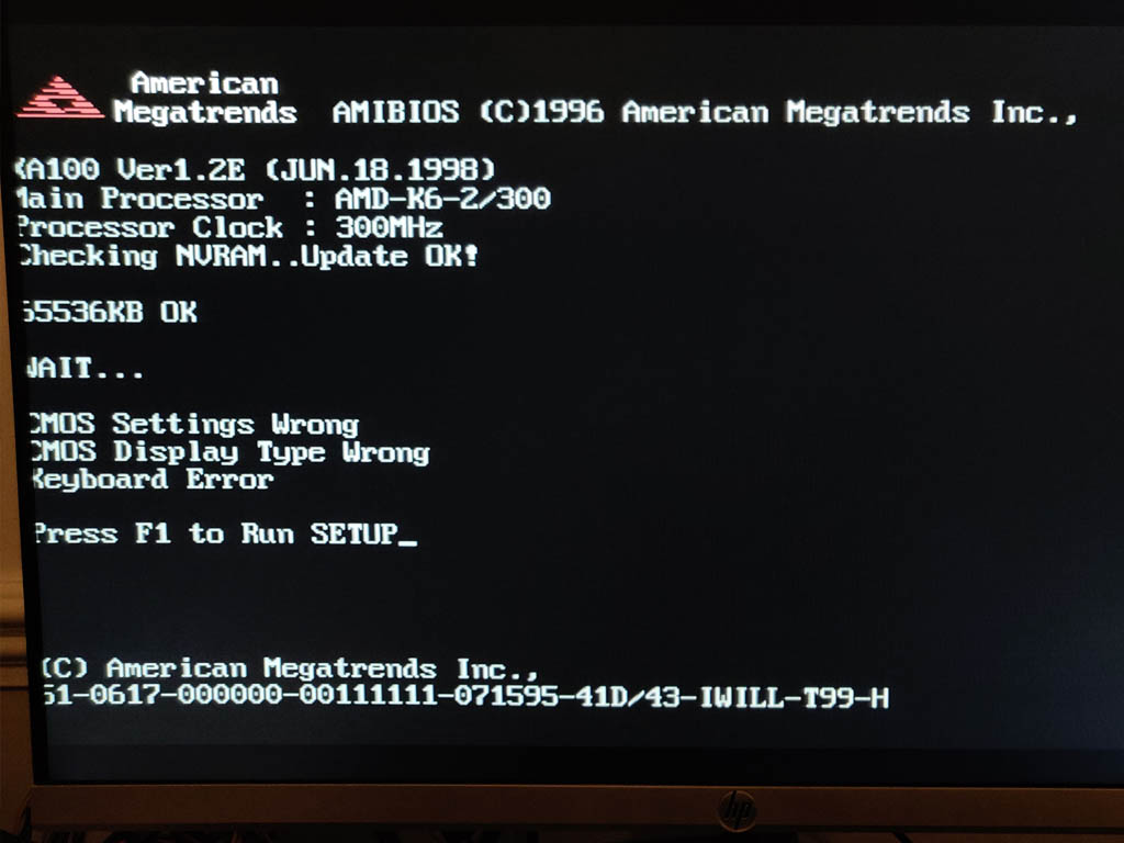
To test the hardware, I powered up the basic components on top of a cardboard box. Generally a good idea and especially so when using older hardware.
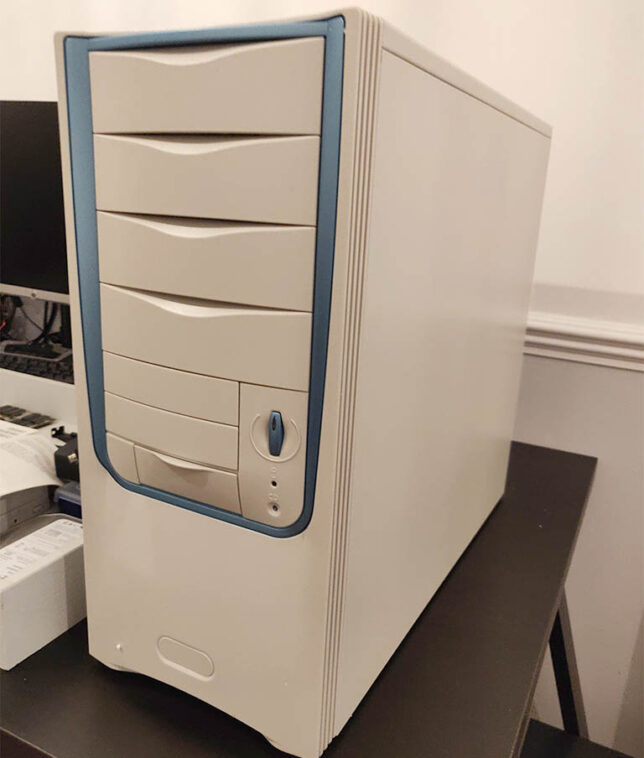
‘Bench’ test of the hardwareFirst POST successful, aside from USB keyboard not working (needed legacy option for USB enabled)The ‘retro’ looking MIDI tower chassis I got for the build
Gaming on the Retro PC Build
After digging out a CD burner and an old image of Windows 98 SE, I’ve got an operating system running and have installed drivers along with a bunch of games.
They play just as I remember. I’ve installed Quake, Quake 2, Unreal Tournament, and a few others to keep me busy for now.
Unreal Tournament in Glide 3dfx rendered mode.
The next step is to replace the temporary modern day LCD monitor I’m using right now. A period correct CRT monitor would really complete the build. I remember Samsung SyncMaster CRTs being excellent. My aim is pick one of these up to complete the system.
If you’re nostalgic like me and want to revisit the PC and games hardware of the late 1990s I highly recommend a build like this.
JSONPath does for JSON processing what XPath (defined as a W3C standard) does for XML. JSONPath queries can be super useful, and are a great addition to any developer or ops person’s toolbox.
You may want to do a quick data query, test, or run through some JSON parsing scenarios for your code. If you have your data easily available in JSON format, then using JSONPath queries or expressions can be a great way to filter your data quickly and efficiently.
JSONPath 101
JSONPath expressions use $ to refer to the outer level object. If for example you have an array at the root, $ would refer to that array.
When writing JSONPath expressions, you can use dot notation or bracket notation. For example:
$.animals.land[0].weight
$['animals']['land'][0]['weight']
You can use filter expressions to filter out specific items in your queries. For example: ?(<bool expression>)
Here is an example that would filter our collection of land animals to show only those heavier than 50.0, returning their names:
$.animals.land[?(@.weight > 50.0)].name
The wildcard character * is used to select all objects or elements.
Note the @ symbol that is used to select the ‘current’ item being iterated in the boolean expression.
There are more JSONPath syntax elements to learn about, but the above are what I find most useful and commonly required.
JSONPath Query Example
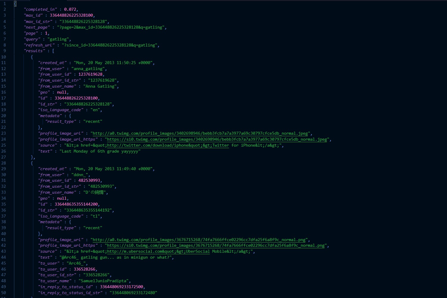
Here is a chunk of JSON data, and some basic queries that show how you can easily filter down the dataset and select what you need.
JSONPath Queries – Example 1
Find all “Report runs” where root.id is equal to a specific value: